The Experiment
Summary
In the experiment we measured the optical transmittance of water vapor using a pair of detectors with different diameters. The objective was to determine whether the transmittance measured with the smaller detector is greater than the transmittance measured with the larger detector. This is one of predictions of the proposed theory.
Two requirements must be met in the experiment. A sufficiently long gas particles mean free path is required. Free from any reactions that could be considered a quantum measurement or lead to decoherence. Therefore, the following should be provided: a large chamber, low pressure, electromagnetic shielding and weak measurement laser light. Secondly, the smaller detector’s light sensitive diameter should be comparable to the standard deviation of the smearing of the tested gas particles wave packets. Even better when it’s smaller. The spread of particles in our chamber is ~13 μm. Diameters of detectors range from 2 μm to 150 μm. In fact, this is the same detector, the effective diameter is controlled by an aperture installed in front of it. The classical, reference detector diameter is 200 μm. A multi-pass Tunable Diode Laser Absorption Spectroscopy type system was used. Transmittance of ~10−2 mbar water vapor on NIR absorption line λ=1368.60 nm was measured using a 60 m long multi-pass cell placed in the 300 l vacuum chamber. Check the 3D visualization.
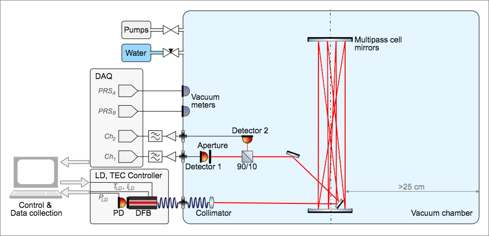
Figure.1 The schematic diagram of the experimental setup.
All optics and detectors are placed inside the vacuum chamber. The electronic equipment and the laser are kept outside.
It took us couple of months to setup the apparatus and perform measurements. We have recorded a few million measurements.
The summarized results of the experiment are presented in the table below. There are the differences in measured transmittances shown for the different detector diameters. The maximum transmittance difference equals to 1.23% and it is observed for the 50μm detector. It may seem not so impressive but there is no other theory explaining any kind of difference of this type. Besides, the statistical significance is greater than 5σ.
| Diameter | Transmittance difference |
|---|---|
| 2 μm | 0.27±0.14 % |
| 5 μm | 0.45±0.12 % |
| 25 μm | 1.36±0.11 % |
| 150 μm | 0.53±0.07 % |
| no aperture (200 μm) | 0.18±0.03 % |
| Diameter | Transmittance difference |
|---|---|
| 2 μm | 0.27 ±0.14 % |
| 5 μm | 0.45 ±0.12 % |
| 15 μm | 0.13 ±0.06 % |
| 25 μm | 0.76 ±0.05 % |
| 40 μm | 0.87 ±0.05 % |
| 50 μm | 1.23 ±0.10 % |
| 100 μm | 0.52 ±0.06 % |
| 150 μm | 0.53 ±0.07 % |
| no aperture (200 μm) | 0.18 ±0.03 % |
Table.1 The aggregated results of the experiment,
a list of transmittance differences measured for different detectors' diameters
The transmittance differences with measurement uncertainties are shown for all detectors' diameters used in the experiment. The most significant results are in bold. The results for 2 μm & 200 μm were measured during two distinct runs. Diameter - the detector (aperture) diameter the transmittance was measured for, Transmittance difference - the mean transmittance difference measured (transmittance difference is equal to transmittance quotient - 1).
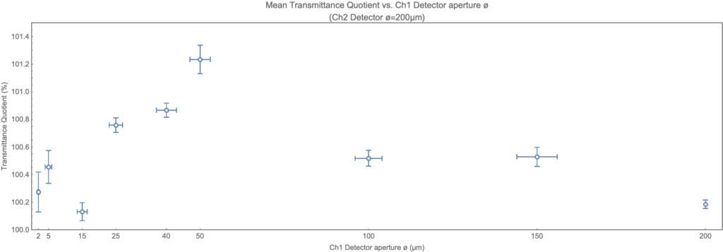
Figure.2 The aggregated results of the experiment.
Mean transmittance quotients TQ along with their 1σ standard errors (vertical bars) and aperture tolerances (horizontal bars). The transmittance quotients are averaged for all pressures for each examined aperture. The rightmost point is the result of no aperture runs.
Classical predictions are that all this differences should be equal and very close to 0. They are not.
This experiment explores new research areas in the field. The objective of the experiment, which is to observe in laboratory conditions the effect predicted by the smeared gas theory, is achieved. It outlines the limits of applicability of the classic Beer-Lamber law.
There is a comprehensive report on the experiment available.
On-line data
There was a lot of data recorded during the experiment. For obvious reasons it can’t fit in the paper report. You can find all recorded data below.
The experiment was carried out in successive runs. There was a different aperture stop installed during each run. A single run takes several days. Each run consists of many consecutive cycles. A single cycle is less than half an hour long. There is a few thousands single measurements in a cycle.
A list of runs is shown in the table below.
| Run name |
Transmittance difference |
Dia |
Duration 2020- |
No. of cycles |
No. of measure |
|
|---|---|---|---|---|---|---|
| R-3 | 0.23 ±0.25 % | 2 μm | Feb 7 Feb 10 |
131 | 384 289 | |
| R-5 | 0.30 ±0.18 % | 2 μm | Feb 25 Mar 1 |
218 | 577 676 | |
| R-6 | 1.36 ±0.11 % | 25 μm | Mar 4 Mar 6 |
71 | 183 212 | |
| R-7 | 0.45 ±0.12 % | 5 μm | Mar 6 Mar 9 |
81 | 214 318 | |
| R-8 | -0.10 ±0.19 % | no aperture (200 μm) |
Mar 10 Mar 11 |
31 | 80 220 | |
| R-9 | 0.53 ±0.07 % | 150 μm | Mar 13 Mar 20 |
268 | 695 544 | |
| R-10 | 0.20 ±0.03 % | no aperture (200 μm) |
Mar 24 Apr 6 |
709 | 1 185 491 | |
| R-11 | 0.13 ±0.06 % | 15 μm | Jun 18 Jun 22 |
558 | 262 717 | |
| R-12 | 0.87 ±0.05 % | 40 μm | Jun 24 Jun 29 |
645 | 303 953 | |
| R-13 | 0.72 ±0.06 % | 25 μm | Jul 01 Jul 10 |
1 177 | 555 846 | |
| R-14 | 1.23 ±0.10 % | 50 μm | Jul 12 Jul 20 |
1 014 | 478 307 | |
| R-15 | 0.52 ±0.06 % | 100 μm | Jul 20 Jul 29 |
1 012 | 479 172 |
Table.2 The list of experiment runs
All experiment runs are presented in the table. Transmittance difference - the mean transmittance difference measured in the run (transmittance difference is equal to transmittance quotient - 1), Diameter - the aperture diameter used during the run, Duration - measurements date range, No. of cycles - the total number of measurement cycles recorded during the run, No. of measurements - the total number of single measuring taken during all cycles, - a link to the run details. page